
Simplified Example Presented In The Paper#
[2]:
# -*- coding: utf-8 -*-
"""
 * Copyright (c) 2023 Alexandre Gauvain, Ronan Abhervé, Jean-Raynald de Dreuzy
 *
 * This program and the accompanying materials are made available under the
 * terms of the Eclipse Public License 2.0 which is available at
 * http://www.eclipse.org/legal/epl-2.0, or the Apache License, Version 2.0
 * which is available at https://www.apache.org/licenses/LICENSE-2.0.
 *
 * SPDX-License-Identifier: EPL-2.0 OR Apache-2.0
"""
[2]:
'\n * Copyright (c) 2023 Alexandre Gauvain, Ronan Abhervé, Jean-Raynald de Dreuzy\n *\n * This program and the accompanying materials are made available under the\n * terms of the Eclipse Public License 2.0 which is available at\n * http://www.eclipse.org/legal/epl-2.0, or the Apache License, Version 2.0\n * which is available at https://www.apache.org/licenses/LICENSE-2.0.\n *\n * SPDX-License-Identifier: EPL-2.0 OR Apache-2.0\n'
[3]:
# PYTHON PACKAGES
import sys
import os
import numpy as np
import pandas as pd
import flopy
import matplotlib as mpl
import matplotlib.pyplot as plt
import matplotlib.dates as mdates
import imageio
import whitebox
wbt = whitebox.WhiteboxTools()
wbt.verbose = False

# ROOT DIRECTORY
from os.path import dirname, abspath
try:
    root_dir = '/home/bb/Documents/01_Git_Repository/01-HydroModPy-dev'
except NameError:
    root_dir = os.getcwd()
sys.path.append(root_dir)

# HYDROMODPY MODULES
from hydromodpy import watershed_root
from hydromodpy.display import visualization_watershed, visualization_results, export_vtuvtk
from hydromodpy.tools import toolbox
fontprop = toolbox.plot_params(8,15,18,20)  # small, medium, interm, large

example_path = os.path.join(root_dir, "examples", "01_simplified_example_presented_in_the_paper/")
data_path = os.path.join(example_path, "data/")

# The folder out_path is created in the example_path root directory:
out_path = os.path.join(root_dir,'examples', 'results')
# Or define it manually
# out_path = 'C:/Simulations/HydroModPy/'

print('The results of the example will be saved here :', out_path)
The results of the example will be saved here : /home/bb/Documents/01_Git_Repository/01-HydroModPy-dev/examples/results
[ ]:
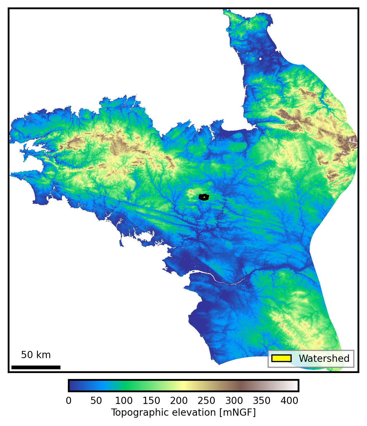
# Name of the study site
watershed_name = 'Example_01_Canut'
print('##### '+watershed_name.upper()+' #####')

# Regional DEM
dem_path = os.path.join(data_path, 'regional dem.tif')

# Outlet coordinates of the catchment
from_xyv = [327816.965, 6777886.670, 150, 10 , 'EPSG:2154']

# Extract the catchment from a regional DEM
BV = watershed_root.Watershed(dem_path=dem_path,
                              out_path=out_path,
                              load=False,
                              watershed_name=watershed_name,
                              from_lib=None, # os.path.join(root_dir,'watershed_library.csv')
                              from_dem=None, # [path, cell size]
                              from_shp=None, # [path, buffer size]
                              from_xyv=from_xyv, # [x, y, snap distance, buffer size]
                              bottom_path=None, # path
                              save_object=True)

# Paths necessary for the script
stable_folder = os.path.join(out_path, watershed_name, 'results_stable')
simulations_folder = os.path.join(out_path, watershed_name, 'results_simulations')
[INFO]       __  __          __           __  ____          ________
[INFO]      / / / /         / /          /  \/   /         / / __  /
[INFO]     / /_/ /_  ______/ /________  /       /___  ____/ / /_/ /_  __
[INFO]    / __  / / / / __  / ___/ __ \/ /\,-/ / __ \/ __  / ____/ / / /
[INFO]   / / / / /_/ / /_/ / /  / /_/ / /   / / /_/ / /_/ / /   / /_/ /
[INFO]  /_/ /_/\__, /_____/_/   \____/_/   /_/\____/_____/_/____\__, /
[INFO]        /____/ Hydrological Modelling in Python /_____________/
[INFO]
[INFO] Initializing watershed object from scratch as requested
[INFO] Extracting geographic data for model area
##### EXAMPLE_01_CANUT #####
[5]:
# General plot of the study site
visualization_watershed.watershed_local(dem_path, BV)
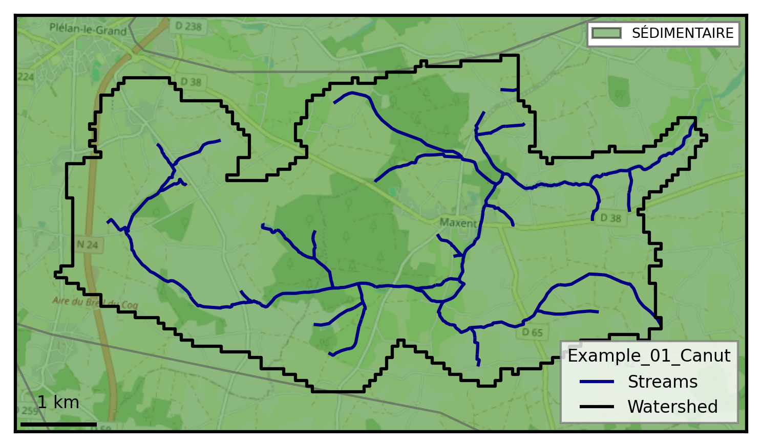
# Clip specific data at the catchment scale
BV.add_geology(data_path, types_obs='GEO1M.shp', fields_obs='CODE_LEG')
BV.add_hydrography(data_path, types_obs=['regional stream network'])
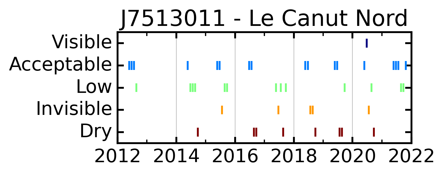
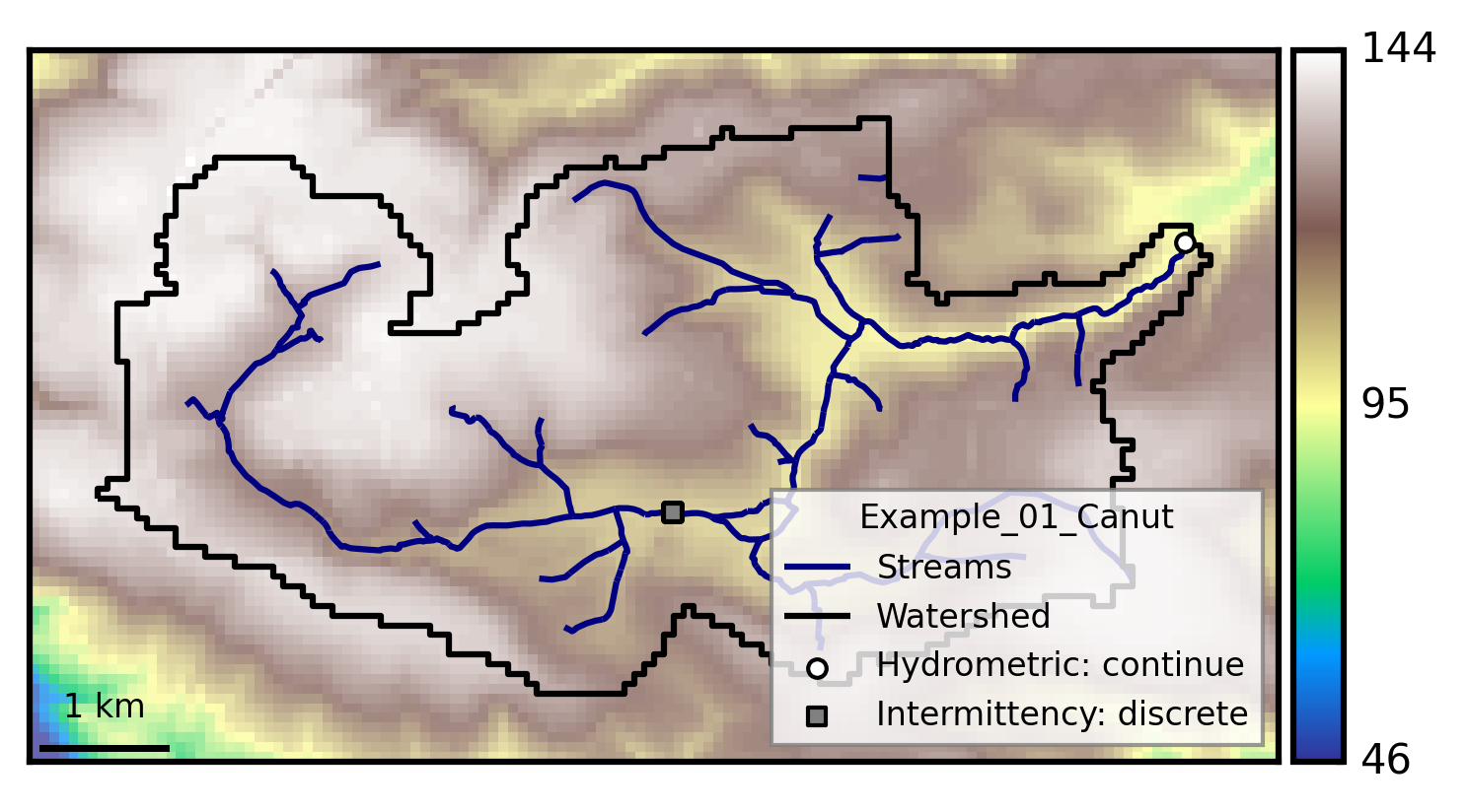
# Add hydrological data
BV.add_hydrometry(data_path, 'france hydrometric stations.shp')
BV.add_intermittency(data_path, 'regional onde stations.shp')
# Extract a subbasin inside the study site
BV.add_subbasin(os.path.join(data_path, 'additional'), 150)
# Visualization
visualization_watershed.watershed_geology(BV)
visualization_watershed.watershed_dem(BV)
[INFO] Extracting geology data from /home/bb/Documents/01_Git_Repository/01-HydroModPy-dev/examples/01_simplified_example_presented_in_the_paper/data/
[INFO] Extracting hydrography data from /home/bb/Documents/01_Git_Repository/01-HydroModPy-dev/examples/01_simplified_example_presented_in_the_paper/data/
[INFO] Extracting hydrometry data from /home/bb/Documents/01_Git_Repository/01-HydroModPy-dev/examples/01_simplified_example_presented_in_the_paper/data/
[INFO] Extracting stream intermittency data from /home/bb/Documents/01_Git_Repository/01-HydroModPy-dev/examples/01_simplified_example_presented_in_the_paper/data/
[INFO] Extracting subbasin definitions for watershed
[6]:
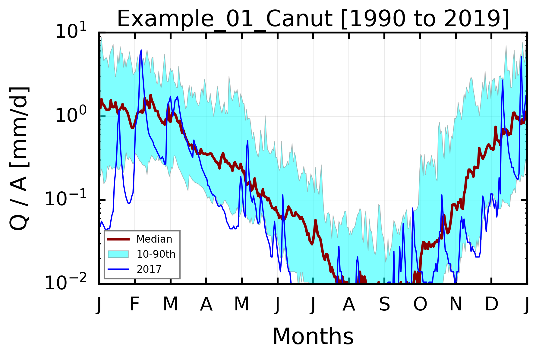
Qobs = pd.read_csv(data_path+'/'+'hydrometry catchment Canut.csv', sep=';', index_col=0, parse_dates=True)
Qobs = Qobs.squeeze()
Qobs = Qobs.rename('Q')
def select_period(df, first, last):
    df = df[(df.index.year>=first) & (df.index.year<=last)]
    return df
area = BV.geographic.area
first = 1990
last = 2019
Qobs = select_period(Qobs, first, last)
Qobs = (Qobs / (area*1000000)) * (3600 * 24) * 1000 # m3/s to mm/j
data_index = Qobs.copy()

mean_mensual = data_index.resample('M').mean() # mensual mean
mean_annual = data_index.resample('Y').mean() # annual mean
Mean = round(data_index.mean(),2)
Mean = data_index.mean()
Min = data_index.resample('Y').min()
Q10 = data_index.resample('Y').quantile(0.10)
Q25 = data_index.resample('Y').quantile(0.25)
Q50 = data_index.resample('Y').quantile(0.50)
Q75 = data_index.resample('Y').quantile(0.75)
Q90 = data_index.resample('Y').quantile(0.90)
Max = data_index.resample('Y').max()
mean_interan_days = data_index.groupby([data_index.index.month,data_index.index.day], as_index=True).mean().to_frame()
std_interan_days = data_index.groupby([data_index.index.month,data_index.index.day], as_index=True).std()
q10_interan_days = data_index.groupby([data_index.index.month,data_index.index.day], as_index=True).quantile(0.10)
q90_interan_days = data_index.groupby([data_index.index.month,data_index.index.day], as_index=True).quantile(0.90)
q50_interan_days = data_index.groupby([data_index.index.month,data_index.index.day], as_index=True).quantile(0.50)
mean_interan_days['std'] = std_interan_days
mean_interan_days['q10'] = q10_interan_days
mean_interan_days['q90'] = q90_interan_days
mean_interan_days['q50'] = q50_interan_days
mean_interan_days.index.names = ['months','days']
mean_interan_days = mean_interan_days.reset_index()
mean_interan_days = mean_interan_days.sort_values(['months','days'])
mean_interan_days['counts'] = np.array(range(1,len(mean_interan_days)+1))

fig, ax = plt.subplots(figsize=(6,4))
ax.plot(mean_interan_days.counts, mean_interan_days.q50, lw=2, color='darkred', label='Median')
yerrmax = mean_interan_days.q90
yerrmin = mean_interan_days.q10
ax.fill_between(mean_interan_days.counts, yerrmin, yerrmax, color='cyan', edgecolor='grey', lw=0.5, alpha=0.5, label='10-90th')
ax.set_yscale('log')
ax.set_xlim(0,366)
ax.set_ylim(0.01,10)
ax.tick_params(axis='both', which='major', pad=10)
x1 = np.linspace(0,366,13)
squad = ['J','F','M','A','M','J','J','A','S','O','N','D','J']
ax.set_xticks(x1)
ax.set_xticklabels(squad, minor=False, rotation='horizontal')
ax.set_xlabel('Months', labelpad=+10)
ax.set_ylabel('Q / A [mm/d]',labelpad=+10)
ax.set_title(watershed_name + ' [' + str(first) + ' to ' + str(last) + ']')
ax.grid(alpha=0.25, zorder=0)
one = 2017
dates = np.array([one],dtype=np.int64)
colors = ['blue']
for z in np.array(range(len(dates))):
    onlyone = data_index[(data_index.index.year==dates[z])].to_frame()
    onlyone = onlyone.groupby([onlyone.index.month, onlyone.index.day], as_index=True).mean()
    onlyone['counts'] = np.array(range(1,len(onlyone)+1))
    ax.plot(onlyone.counts, onlyone['Q'], color=colors[z], lw=1, label = str(dates[z]))
ax.legend(loc='lower left')
plt.tight_layout()
[7]:
# Name of the model/simulation
model_name = 'test_0'

# Import modules
BV.add_settings()
BV.add_climatic()
BV.add_hydraulic()

# Frame settings
BV.settings.update_model_name(model_name) # Name of the model/simulation
BV.settings.update_box_model(True)
BV.settings.update_sink_fill(False)
BV.settings.update_simulation_state('steady') # Transient
BV.settings.update_check_model(plot_cross=False, check_grid=True)
BV.settings.update_dis_perlen(dis_perlen=False)

# Climatic settings
BV.climatic.update_recharge(350 / 1000 / 365, sim_state=BV.settings.sim_state)
BV.climatic.update_first_clim('mean') # or 'first or value

# Hydraulic settings
BV.hydraulic.update_nlay(5)
BV.hydraulic.update_lay_decay(1.5) # 1 if not activated
BV.hydraulic.update_bottom(None) # Set a value to set a flat bottom
BV.hydraulic.update_thick(50) # Not consider if bottom != of None
BV.hydraulic.update_hk(2e-5 * 24 * 3600) # m/d
BV.hydraulic.update_sy(1/100) # -
BV.hydraulic.update_hk_decay(1/20, min_value=None, log_transf=False) # Exponential decay with depth : 1/10 (about half decrease at 10m)
BV.hydraulic.update_sy_decay(1/20, min_value=None, log_transf=False)
BV.hydraulic.update_ss_decay(1/20, min_value=None, log_transf=False)
BV.hydraulic.update_hk_vertical(None) # or [ [1e-5, [0, 20]], [1e-6, [20,80]] ]
BV.hydraulic.update_cond_drain(None)

# Boundary settings
BV.settings.update_bc_sides(None, None)
BV.add_oceanic('None')

# Particle tracking settings
BV.settings.update_input_particles(zone_partic = os.path.join(simulations_folder,model_name,'_postprocess/_rasters/seepage_areas_t(0).tif'),
                                   track_dir = 'backward')
[INFO] Initializing settings module for groundwater parameters
[INFO] Initializing climatic module parameters
[INFO] Initializing hydraulic module for parameter setup
[ ]:
# Pre-processing
model_modflow = BV.preprocessing_modflow(for_calib=False)

# Processing
success_modflow = BV.processing_modflow(model_modflow, write_model=True, run_model=True)

# Post-processing
if success_modflow == True:
    BV.postprocessing_modflow(model_modflow,
                              watertable_elevation=True,
                              watertable_depth=True,
                              seepage_areas=True,
                              outflow_drain=True,
                              groundwater_flux=True,
                              groundwater_storage=True,
                              accumulation_flux=True,
                              persistency_index=False, # only in transient
                              intermittency_monthly=False, # only in transient
                              intermittency_weekly=False, # only in transient
                              intermittency_daily=False, # only in transient
                              export_all_tif=False)
[WARNING] MODFLOW grid connectivity check found 78 problematic cells
FloPy is using the following executable to run the model: ../../../../../bin/linux/mfnwt

                                  MODFLOW-NWT-SWR1
    U.S. GEOLOGICAL SURVEY MODULAR FINITE-DIFFERENCE GROUNDWATER-FLOW MODEL
                             WITH NEWTON FORMULATION
                             Version 1.3.0 07/01/2022
                    BASED ON MODFLOW-2005 Version 1.12.0 02/03/2017

                    SWR1 Version 1.05.0 03/10/2022

 Using NAME file: test_0.nam
 Run start date and time (yyyy/mm/dd hh:mm:ss): 2025/11/12  1:43:38

 Solving:  Stress period:     1    Time step:     1    Groundwater-Flow Eqn.
[INFO] Post-processing stress period 1/1
 Run end date and time (yyyy/mm/dd hh:mm:ss): 2025/11/12  1:43:38
 Elapsed run time:  0.786 Seconds

  Normal termination of simulation
[INFO] Exporting watertable elevation time series
[INFO] Exporting watertable depth time series
[INFO] Exporting seepage areas time series
[INFO] Exporting outflow drain time series
[INFO] Exporting groundwater flux time series
[INFO] Exporting groundwater storage time series
[INFO] Exporting accumulation flux time series
[9]:
# Pre-processing
if success_modflow == True:
    model_modpath = BV.preprocessing_modpath(model_modflow)

# Processing
    success_modpath = BV.processing_modpath(model_modpath, write_model=True, run_model=True)

# Post-processing
if success_modpath == True:
    BV.postprocessing_modpath(model_modpath,
                              ending_point=True,
                              starting_point=True,
                              pathlines_shp=True,
                              particles_shp=False,
                              random_id=None) # None
writing loc particle data
FloPy is using the following executable to run the model: ../../../../../bin/linux/mp6
Processing basic data ...
Checking head file ...
Checking budget file and building index ...

Run particle tracking simulation ...
Processing Time Step     1 Period     1.  Time =  1.00000E+00
Particle tracking complete. Writing endpoint file ...
End of MODPATH simulation. Normal termination.
(numpy.record, [('particleid', '<i4'), ('particlegroup', '<i4'), ('timepointindex', '<i4'), ('cumulativetimestep', '<i4'), ('time', '<f4'), ('x', '<f4'), ('y', '<f4'), ('z', '<f4'), ('k', '<i4'), ('i', '<i4'), ('j', '<i4'), ('grid', '<i4'), ('xloc', '<f4'), ('yloc', '<f4'), ('zloc', '<f4'), ('linesegmentindex', '<i4')])
[10]:
timeseries_results = BV.postprocessing_timeseries(model_modflow=model_modflow,
                                                  model_modpath=model_modpath,
                                                  subbasin_results=True,
                                                  datetime_format=False)
[INFO] Exported catchment time series to /home/bb/Documents/01_Git_Repository/01-HydroModPy-dev/examples/results/Example_01_Canut/results_simulations/test_0/_postprocess/_timeseries
[INFO] Exported time series for subbasin 1 to /home/bb/Documents/01_Git_Repository/01-HydroModPy-dev/examples/results/Example_01_Canut/results_simulations/test_0/_subbasins/hydrometry_J7513010
[INFO] Exported time series for subbasin 2 to /home/bb/Documents/01_Git_Repository/01-HydroModPy-dev/examples/results/Example_01_Canut/results_simulations/test_0/_subbasins/intermittency_J7513011
[INFO] Exported time series for subbasin 3 to /home/bb/Documents/01_Git_Repository/01-HydroModPy-dev/examples/results/Example_01_Canut/results_simulations/test_0/_subbasins/subbasin_Upstream
[11]:
netcdf_results = BV.postprocessing_netcdf(model_modflow,
                                          datetime_format=False)
[INFO] Exporting MODFLOW results as NetCDF for model test_0
[12]:
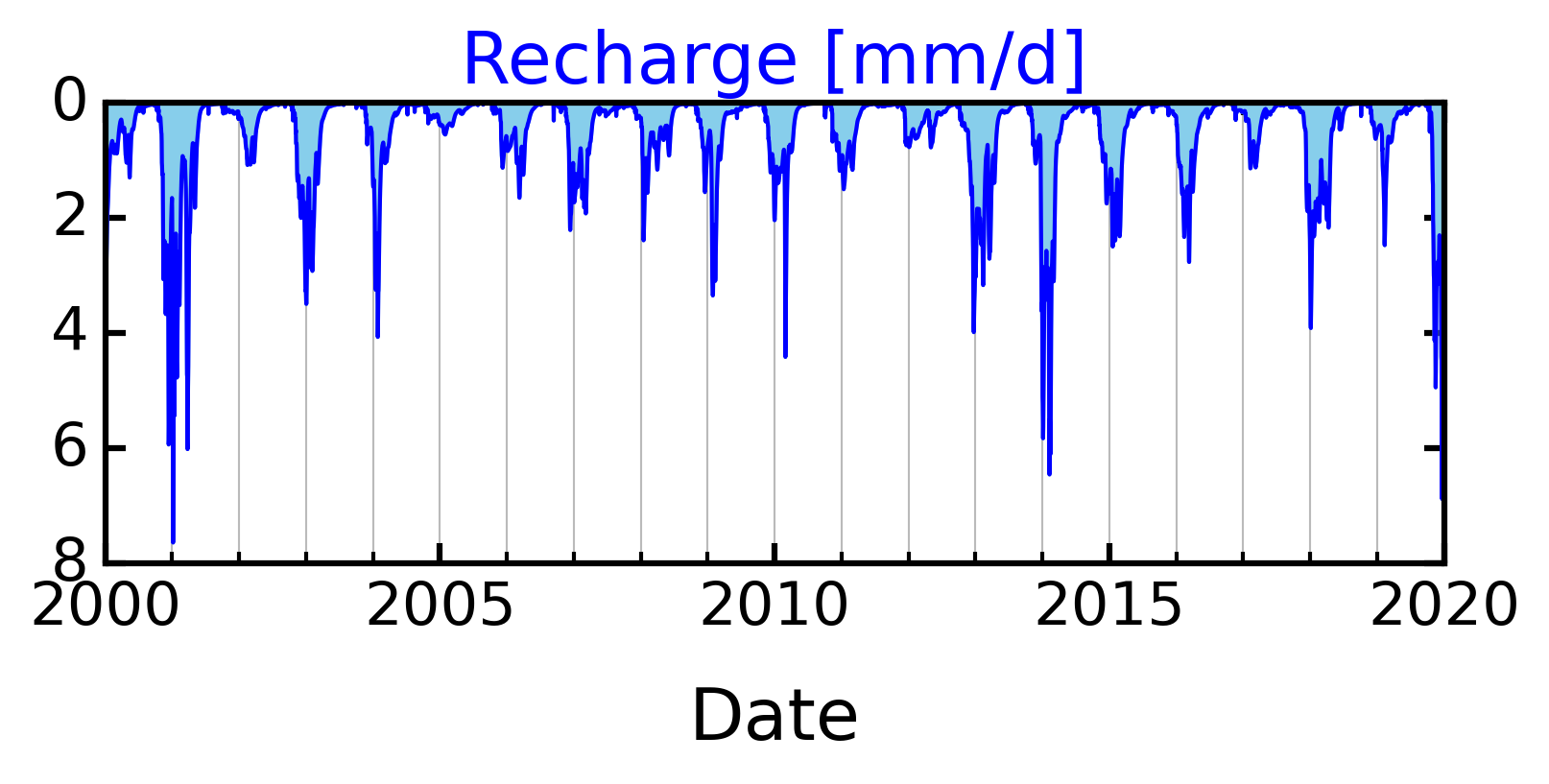
BV.add_climatic()
BV.climatic.update_recharge_reanalysis(path_file=os.path.join(data_path,'_climate_REANALYSIS.csv'),
                                       clim_mod='REA',
                                       clim_sce='historic',
                                       first_year=1990,
                                       last_year=2019,
                                       time_step='D',
                                       sim_state='transient')

fig, ax = plt.subplots(1,1, figsize=(6,2), dpi=300)
ax.patch.set_visible(False)
# axb = ax.twinx()
R = BV.climatic.recharge
ax.plot(R.index, R,  color='blue', lw=1, ms=0, clip_on=True)
# axb.bar(R.resample('Y').sum().index, R.resample('Y').sum(),  color='red', lw=0, width=100, alpha=1, clip_on=True)
# axb.set_ylim(0,1000)
# axb.invert_yaxis()
ax.fill_between(R.index, R*0, R, color='skyblue', clip_on=True, alpha=1)
ax.set_xlabel('Date')
# ax.set_ylabel('Recharge [mm/d]', color='blue')
ax.xaxis.set(minor_locator=mdates.YearLocator(1), major_locator=mdates.YearLocator(5))
ax.set_ylim(0,8)
ax.set_xlim(pd.to_datetime('2000'), pd.to_datetime('2020'))
ax.set_yticks([0,2,4,6,8])
ax.grid(which='both', axis='x')
# ax.set_zorder(axb.get_zorder() + 1)
# plt.setp(axb.get_yticklabels(), color="red")
ax.invert_yaxis()
ax.set_title('Recharge [mm/d]', color='blue')

# fig.savefig(out_path+'/'+watershed_name+'/results_simulations/'+model_name+'/_postprocess/_figures/'+'input_rec.png', dpi=300, bbox_inches='tight')
[INFO] Initializing climatic module parameters
[12]:
Text(0.5, 1.0, 'Recharge [mm/d]')
[ ]:
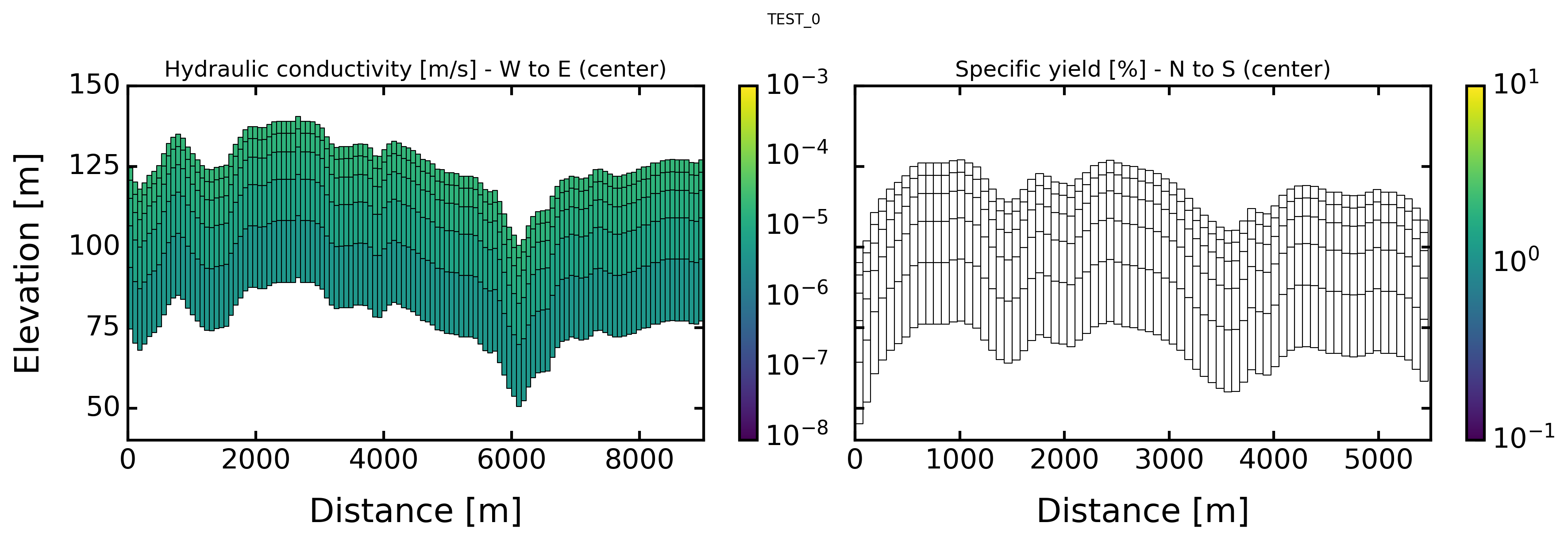
mf = flopy.modflow.Modflow.load(simulations_folder+'/'+model_name+'/'+model_name+'.nam')
gridname = simulations_folder+model_name+'/'+model_name+'.dis'
grid_model = mf.modelgrid
hk_grid = mf.upw.hk
sy_grid = mf.upw.sy

fig, axs = plt.subplots(1, 2, figsize=(12, 4), sharey=True)
axs = axs.ravel()

ax = axs[0]
modelxsect = flopy.plot.PlotCrossSection(model=mf, line={'Row': int((grid_model.shape[1])/2)})
val = hk_grid.array/24/3600 # m/s
try:
    for i in range(val.shape[0]):
        val[i][val[i] <= np.nanmin(val[i])] = np.nanmin(val[i][np.nonzero(val[i])])
except:
    pass
cb = modelxsect.plot_array(val, ax=ax, cmap='viridis', lw=0.5, norm=mpl.colors.LogNorm(vmin=1e-3,vmax=1e-8))
ax.set_title('Hydraulic conductivity [m/s] - W to E (center)', fontsize=12)
ax.set_xlim(0, 9000)
ax.set_ylim(40, 150)
ax.set_xticks([0,2000,4000,6000,8000])
ax.set_yticks([50,75,100,125,150])
ax.set_xlabel('Distance [m]')
ax.set_ylabel('Elevation [m]')
fig.suptitle(model_name.upper(), x=0.22, y=1.05, fontsize=8)
fig.colorbar(cb)
plt.tight_layout()

ax = axs[1]
modelxsect = flopy.plot.PlotCrossSection(model=mf, line={'Column': int((grid_model.shape[2])/2)})
cb = modelxsect.plot_array(sy_grid.array*100, ax=ax, cmap='viridis', lw=0.5,
                            # vmin=0, vmax=30,
                            norm=mpl.colors.LogNorm(vmin=0.1,
                                                    vmax=10))
ax.set_title('Specific yield [%] - N to S (center)', fontsize=12)
ax.set_xlim(0, 5500)
ax.set_ylim(40, 150)
ax.set_xticks([0,1000,2000,3000,4000,5000])
ax.set_yticks([50,75,100,125,150])
ax.set_xlabel('Distance [m]')
fig.suptitle(model_name.upper(), x=0.5, y=1.0, fontsize=8)
fig.colorbar(cb)
plt.tight_layout()

# fig.savefig(out_path+'/'+watershed_name+'/results_simulations/'+model_name+'/_postprocess/_figures/'+'mesh_cross.png', dpi=300, bbox_inches='tight')
[ ]:
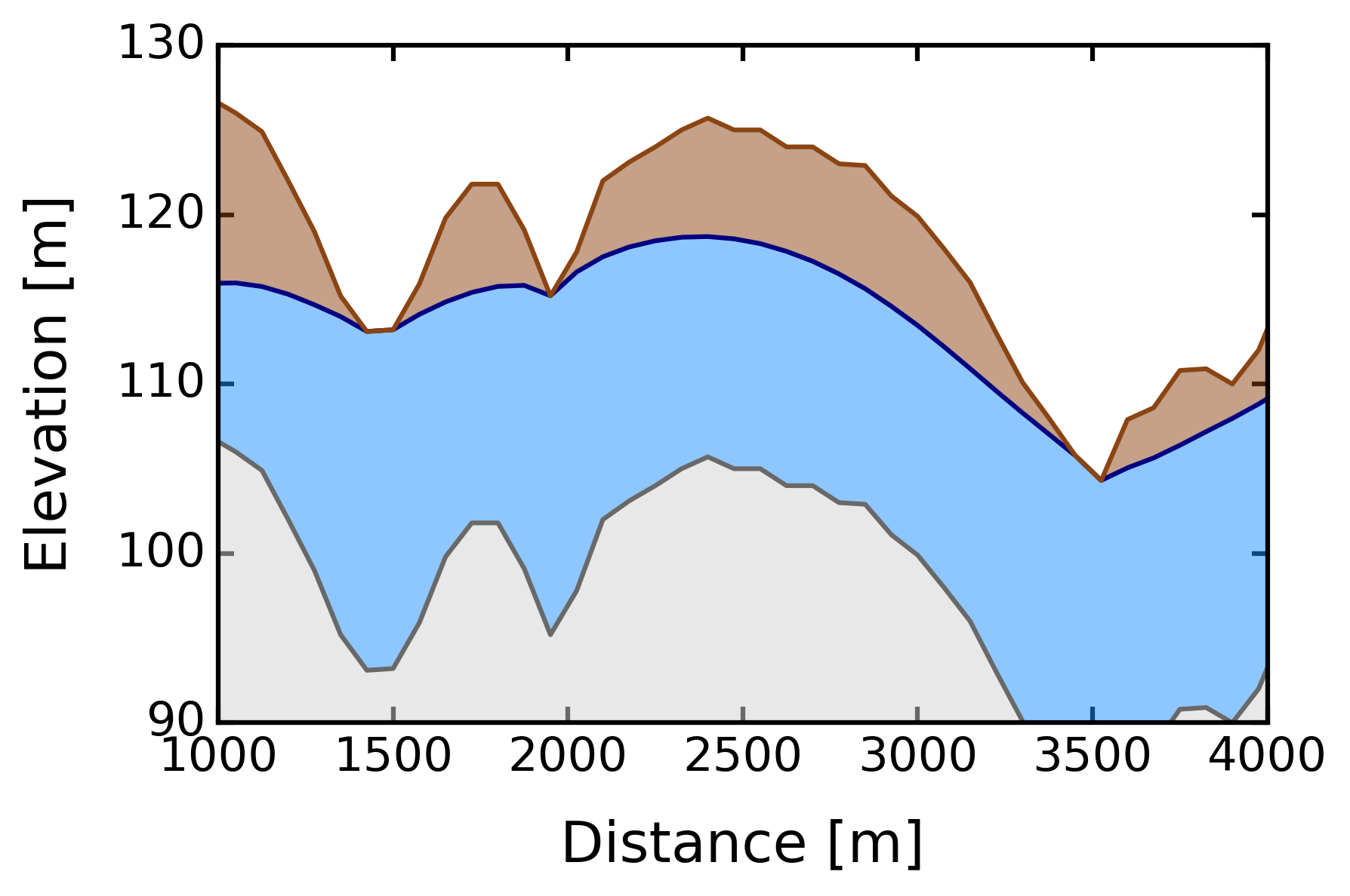
fig, ax = plt.subplots(1, 1, figsize=(6,4), dpi=300)
print(stable_folder)

mask = imageio.imread(stable_folder+'/geographic/'+'watershed_dem.tif')
watertable_elevation = np.load(simulations_folder+'/'+model_name+'/_postprocess/'+'watertable_elevation'+'.npy', allow_pickle=True).item()

dem_data = imageio.imread(BV.geographic.watershed_dem)
wt_data = watertable_elevation[0]

xvalues = np.linspace(-1,1,dem_data.shape[1])
yvalues = np.linspace(-1,1,dem_data.shape[0])
xx, yy = np.meshgrid(xvalues,yvalues)

cur_x = dem_data.shape[1] /2
cur_x = 65

wt_prof = wt_data.astype(float)
wt_prof[wt_prof<0] = np.nan
dem_max = dem_data.max()
dem_prof = dem_data.astype(float)
dem_prof[dem_prof<0] = np.nan
dem_plot = np.ma.masked_array(dem_data, mask=(dem_data<0))
dem_v_plot = dem_prof[:,int(cur_x)]
dem_v_plot[dem_v_plot == 0] = np.nan
wt_v_plot = wt_prof[:,int(cur_x)]
wt_v_plot[wt_v_plot == 0] = np.nan

wt_v_fill = ax.fill_between(np.arange(xx.shape[0])*75, dem_v_plot-20, wt_v_plot, color='dodgerblue', alpha=0.5, lw=0)
w_prof = ax.plot(np.arange(xx.shape[0])*75, wt_v_plot, color='navy', lw=1.5)
wt_v_fill = ax.fill_between(np.arange(xx.shape[0])*75, wt_v_plot, dem_v_plot, color='saddlebrown', alpha=0.5, lw=0)
d_prof = ax.plot(np.arange(xx.shape[0])*75, dem_v_plot, 'saddlebrown', lw=1.5)
ax.fill_between(np.arange(xx.shape[0])*75, 0, dem_v_plot-20, color='lightgrey', alpha=0.5, lw=0)
ax.plot(np.arange(xx.shape[0])*75, dem_v_plot-20, color='dimgray', lw=1.5)

ax.set_xlim(1000, 4000)
ax.set_ylim(90, 130)
ax.set_yticks([90,100,110,120,130])
ax.set_xlabel('Distance [m]')
ax.set_ylabel('Elevation [m]')

plt.tight_layout()

# fig.savefig(out_path+'/'+watershed_name+'/results_simulations/'+model_name+'/_postprocess/_figures/'+'2D_cross.png', dpi=300, bbox_inches='tight')
/home/bb/Documents/01_Git_Repository/01-HydroModPy-dev/examples/results/Example_01_Canut/results_stable
[ ]:
visu = visualization_results.Visualization(BV, model_name)
visu.visual2D(object_list = [
                             'map',
                             'grid',
                             'watertable',
                             'watertable_depth',
                             'drain_flow',
                             'surface_flow',
                             'pathlines',
                             'residence_times'
                             ],
              color_scale = [
                             (None,None),
                             (80,150),
                             (80,150),
                             (0,10),
                             (0,200),
                             (0,30000),
                             (0,3),
                             (0,3),
                             ],
                             lines=1000)
[INFO] Plotting 2D map visualizations for model test_0

[16]:
export_vtuvtk.VTK(BV, model_name)
visu = visualization_results.Visualization(BV, model_name)
visu.visual3D(interactive=True, object_list=[
                                             'grid',
                                             'watertable',
                                             'watertable_depth',
                                             'surface_flow',
                                             'drain_flow',
                                             'pathlines'
                                             ],
                                               view='south-west',
                                              # view='north',
                                              lines=None,
                                              cloc=(0.7,0.1),
                                              z_scale=10)
[INFO] Exporting VTU/VTK grid mesh for model test_0
[INFO] Exporting VTU/VTK water table surfaces for model test_0
[INFO] Exporting VTU/VTK watershed boundary for model test_0
[INFO] Exported VTU/VTK pathlines for model test_0
[ERROR] Failed to export VTU/VTK piezometers for model test_0
Traceback (most recent call last):
  File "/home/bb/Documents/01_Git_Repository/01-HydroModPy-dev/hydromodpy/display/export_vtuvtk.py", line 118, in __init__
    self.piezometers(save_file, watershed.piezometry)
                                ^^^^^^^^^^^^^^^^^^^^
AttributeError: 'Watershed' object has no attribute 'piezometry'. Did you mean: 'add_piezometry'?
[INFO] Exported VTU/VTK streams for model test_0
[INFO] Plotting 3D visualization for model test_0
[INFO] Processing object grid
[INFO] Processing object watertable
[INFO] Processing object watertable_depth
[INFO] Processing object surface_flow
[INFO] Processing object drain_flow
[INFO] Processing object pathlines
[17]:
# CLICK on the map to select a cross-section !
dem_data = imageio.imread(os.path.join(stable_folder,'geographic','watershed_box_buff_dem.tif')) # dem data
stream_data = imageio.imread(os.path.join(stable_folder,'hydrography','regional stream network.tif')) # river data
watertable_data = imageio.imread(os.path.join(simulations_folder,model_name,'_postprocess/_rasters/','watertable_elevation_t(0).tif')) # watertable data
interactive = True
visu = visualization_results.Visualization(BV, model_name)
visu.interactive_cross_section(dem_data, watertable_data, stream_data, interactive)
[INFO] Plotting 2D cross-section for model test_0
[INFO] Matplotlib interactive backend enabled: QtAgg
[ ]:
os.chdir(root_dir)

# %%