
Quick Test Of Wide Hydromodpy Capabilities#
[2]:
# -*- coding: utf-8 -*-
"""
 * Copyright (c) 2023 Alexandre Gauvain, Ronan Abhervé, Jean-Raynald de Dreuzy
 *
 * This program and the accompanying materials are made available under the
 * terms of the Eclipse Public License 2.0 which is available at
 * http://www.eclipse.org/legal/epl-2.0, or the Apache License, Version 2.0
 * which is available at https://www.apache.org/licenses/LICENSE-2.0.
 *
 * SPDX-License-Identifier: EPL-2.0 OR Apache-2.0
"""
[2]:
'\n * Copyright (c) 2023 Alexandre Gauvain, Ronan Abhervé, Jean-Raynald de Dreuzy\n *\n * This program and the accompanying materials are made available under the\n * terms of the Eclipse Public License 2.0 which is available at\n * http://www.eclipse.org/legal/epl-2.0, or the Apache License, Version 2.0\n * which is available at https://www.apache.org/licenses/LICENSE-2.0.\n *\n * SPDX-License-Identifier: EPL-2.0 OR Apache-2.0\n'
[3]:
# PYTHON PACKAGES
import sys
import os
import warnings
import numpy as np
import pandas as pd
import matplotlib as mpl
import matplotlib.pyplot as plt
import matplotlib.dates as mdates
import imageio
import whitebox
import rasterio
import geopandas as gpd
from mpl_toolkits.axes_grid1 import make_axes_locatable
wbt = whitebox.WhiteboxTools()
wbt.verbose = False

# ROOT DIRECTORY
from os.path import dirname, abspath
try:
    root_dir = '/home/bb/Documents/01_Git_Repository/01-HydroModPy-dev'
except NameError:
    root_dir = os.getcwd()
sys.path.append(root_dir)

# HYDROMODPY MODULES
from hydromodpy import watershed_root
from hydromodpy.display import visualization_watershed, visualization_results
from hydromodpy.tools import toolbox
fontprop = toolbox.plot_params(8,15,18,20) # small, medium, interm, large
[4]:
# By default, HydroModPy logs INFO messages to console and creates a debug log
# file in the watershed output folder. You can customize this behavior:

from hydromodpy import log_manager

# Change console output level (default is "verbose")
# log_manager.set_console_level("quiet")    # Only show warnings and errors
# log_manager.set_console_level("verbose")  # Show info, warnings, and errors
# log_manager.set_console_level("dev")      # Show everything including debug

# Enable user log file in current directory (optional)
# log_manager.enable_user_log()                           # Save to current directory
# log_manager.enable_user_log("/path/to/your/folder")    # Save to specific path

# Show logs from third-party libraries (fiona, rasterio, matplotlib, etc.)
# By default, these libraries are muted to avoid cluttering the console
# log_manager.show_library_logs(True)    # Show library warnings
# log_manager.show_library_logs(False)   # Hide library logs (default)

# Note: A complete debug log is automatically saved in the watershed output folder
# at: out_path/watershed_name/hydromodpy_debug.log
[5]:
regression_path = os.path.join(root_dir, "examples", "00_quick_test_of_wide_hydromodpy_capabilities/")
data_path = os.path.join(regression_path, "data/")

# The folder out_path is created in the example_path root directory:
out_path = os.path.join(root_dir, "examples", "results")
# Or define it manually
# out_path = 'D:/_HydroModPy/_results'

print('The results of the example will be saved here :', out_path)
The results of the example will be saved here : /home/bb/Documents/01_Git_Repository/01-HydroModPy-dev/examples/results
[ ]:
# Name of the study site
watershed_name = 'Example_00_Aber'
print('##### '+watershed_name.upper()+' #####')

# Regional DEM
dem_path = os.path.join(data_path, 'regional dem.tif')

# Outlet coordinates of the catchment
from_xyv = [150727.164, 6858066.520, 100, 10 , 'EPSG:2154']

# Extract the catchment from a regional DEM
BV = watershed_root.Watershed(dem_path=dem_path,
                              out_path=out_path,
                              load=False,
                              watershed_name=watershed_name,
                              from_lib=None, # os.path.join(root_dir,'watershed_library.csv')
                              from_dem=None, # [path, cell size]
                              from_shp=None, # [path, buffer size]
                              from_xyv=from_xyv, # [x, y, snap distance, buffer size]
                              bottom_path=None, # path
                              save_object=True)

# Paths necessary for the script
stable_folder = os.path.join(out_path, watershed_name, 'results_stable')
simulations_folder = os.path.join(out_path, watershed_name, 'results_simulations')
[INFO]       __  __          __           __  ____          ________
[INFO]      / / / /         / /          /  \/   /         / / __  /
[INFO]     / /_/ /_  ______/ /________  /       /___  ____/ / /_/ /_  __
[INFO]    / __  / / / / __  / ___/ __ \/ /\,-/ / __ \/ __  / ____/ / / /
[INFO]   / / / / /_/ / /_/ / /  / /_/ / /   / / /_/ / /_/ / /   / /_/ /
[INFO]  /_/ /_/\__, /_____/_/   \____/_/   /_/\____/_____/_/____\__, /
[INFO]        /____/ Hydrological Modelling in Python /_____________/
[INFO]
[INFO] Initializing watershed object from scratch as requested
[INFO] Extracting geographic data for model area
##### EXAMPLE_00_ABER #####
[7]:
# Clip specific data at the catchment scale
BV.add_hydrography(data_path, types_obs=['regional stream network'])
[INFO] Extracting hydrography data from /home/bb/Documents/01_Git_Repository/01-HydroModPy-dev/examples/00_quick_test_of_wide_hydromodpy_capabilities/data/
[8]:
# Name of the model/simulation
model_name = 'reg_0'
# Import modules
BV.add_settings()
BV.add_climatic()
BV.add_hydraulic()
BV.add_oceanic('None')
# Frame settings
BV.settings.update_model_name(model_name) # Name of the model/simulation
BV.settings.update_box_model(True)
BV.settings.update_sink_fill(False)
BV.settings.update_simulation_state('transient') # steady
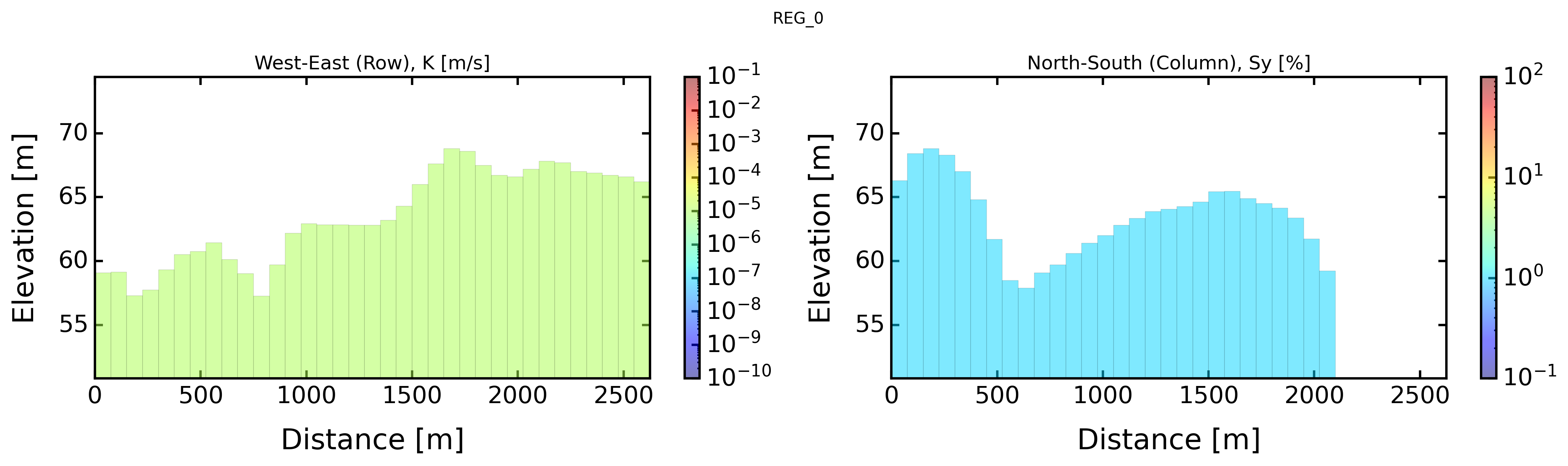
BV.settings.update_check_model(plot_cross=True, check_grid=True)
BV.settings.update_dis_perlen(dis_perlen=True)
# Climatic settings
time_index = pd.date_range(start='2017-01-01', end='2017-12-31', freq='M') # datetime in months
rch_series = pd.Series([10, 60, 40, 20, 10, 5, 4, 20, 10, 1, 0, 0]) / 1000 / 30 # recharge mm/month to in m/day
recharge = pd.Series(rch_series.values, index=time_index)
BV.climatic.update_recharge(recharge, sim_state=BV.settings.sim_state)
BV.climatic.update_runoff(None, sim_state=BV.settings.sim_state)
BV.climatic.update_first_clim('mean') # or 'first or value
# Well settings
well_1_coords = [1-1,9-1,29-1] # [lay, row, col]
well_2_coords = [1-1,17-1,29-1] # [lay, row, col]
well_1_fluxes = pd.Series([-200, 0, -100, 0, 0, 0, 0, 0, 0, 0, 0, 0]) # [L3/T]
well_2_fluxes = pd.Series([-500, 0, 0, -500, 0, 0, -500, 0, 0, 0, 0, 0]) # [L3/T]
BV.settings.update_well_pumping(well_coords=[well_1_coords, well_2_coords],
well_fluxes=[well_1_fluxes, well_2_fluxes])
# Hydraulic settings
BV.hydraulic.update_bottom(None) # Set a value to set a flat bottom
BV.hydraulic.update_thick(50) # Not consider if bottom != of None
BV.hydraulic.update_nlay(1)
BV.hydraulic.update_lay_decay(1) # 1 if not activated
BV.hydraulic.update_hk(1e-5 * 24 * 3600) # m/d
BV.hydraulic.update_sy(1/100) # -
BV.hydraulic.update_ss(1e-5) # -
BV.hydraulic.update_hk_decay(0, None, False) # alpha, kmin, log_transf
BV.hydraulic.update_sy_decay(0, None, False)
BV.hydraulic.update_ss_decay(0, None, False)
BV.hydraulic.update_hk_vertical(None) # or [ [1e-5, [0, 20]], [1e-6, [20,80]] ]
BV.hydraulic.update_sy_vertical(None) # or [ [1e-5, [0, 20]], [1e-6, [20,80]] ]
BV.hydraulic.update_vka(1) # anisotropy ratio Kxy/Kz
BV.hydraulic.update_cond_drain(None)
# Boundary settings
BV.settings.update_bc_sides(None, None)
# Particle tracking settings
BV.settings.update_input_particles(zone_partic = os.path.join(simulations_folder,model_name,'_postprocess/_rasters/seepage_areas_t(0).tif'),
cell_div = 1, # 1
zloc_div = False, # True or False, add cells in vertical
bore_depth = None, # True or None, inject in each lay
track_dir = 'backward',
sel_random = None, # or int
sel_slice = None, # or int
)
[INFO] Initializing settings module for groundwater parameters
[INFO] Initializing climatic module parameters
[INFO] Initializing hydraulic module for parameter setup
[ ]:
# Pre-processing
model_modflow = BV.preprocessing_modflow(for_calib=False)

# Processing
success_modflow = BV.processing_modflow(model_modflow, write_model=True, run_model=True)

# Post-processing
BV.postprocessing_modflow(model_modflow,
                          watertable_elevation=True,
                          watertable_depth=True,
                          seepage_areas=True,
                          outflow_drain=True,
                          groundwater_flux=True,
                          groundwater_storage=True,
                          accumulation_flux=True,
                          persistency_index=True, # only in transient
                          intermittency_monthly=True, # only in transient
                          intermittency_weekly=False, # only in transient
                          intermittency_daily=False, # only in transient
                          export_all_tif=True)

BV.postprocessing_netcdf(model_modflow,
                         datetime_format=False)
[INFO] MODFLOW grid connectivity check passed
[INFO] Post-processing stress period 1/12
FloPy is using the following executable to run the model: ../../../../../bin/linux/mfnwt

                                  MODFLOW-NWT-SWR1
    U.S. GEOLOGICAL SURVEY MODULAR FINITE-DIFFERENCE GROUNDWATER-FLOW MODEL
                             WITH NEWTON FORMULATION
                             Version 1.3.0 07/01/2022
                    BASED ON MODFLOW-2005 Version 1.12.0 02/03/2017

                    SWR1 Version 1.05.0 03/10/2022

 Using NAME file: reg_0.nam
 Run start date and time (yyyy/mm/dd hh:mm:ss): 2025/11/12  1:49:04

 Solving:  Stress period:     1    Time step:     1    Groundwater-Flow Eqn.
 Solving:  Stress period:     2    Time step:     1    Groundwater-Flow Eqn.
 Solving:  Stress period:     3    Time step:     1    Groundwater-Flow Eqn.
 Solving:  Stress period:     4    Time step:     1    Groundwater-Flow Eqn.
 Solving:  Stress period:     5    Time step:     1    Groundwater-Flow Eqn.
 Solving:  Stress period:     6    Time step:     1    Groundwater-Flow Eqn.
 Solving:  Stress period:     7    Time step:     1    Groundwater-Flow Eqn.
 Solving:  Stress period:     8    Time step:     1    Groundwater-Flow Eqn.
 Solving:  Stress period:     9    Time step:     1    Groundwater-Flow Eqn.
 Solving:  Stress period:    10    Time step:     1    Groundwater-Flow Eqn.
 Solving:  Stress period:    11    Time step:     1    Groundwater-Flow Eqn.
 Solving:  Stress period:    12    Time step:     1    Groundwater-Flow Eqn.
 Run end date and time (yyyy/mm/dd hh:mm:ss): 2025/11/12  1:49:04
 Elapsed run time:  0.113 Seconds

  Normal termination of simulation
[INFO] Post-processing stress period 2/12
[INFO] Post-processing stress period 3/12
[INFO] Post-processing stress period 4/12
[INFO] Post-processing stress period 5/12
[INFO] Post-processing stress period 6/12
[INFO] Post-processing stress period 7/12
[INFO] Post-processing stress period 8/12
[INFO] Post-processing stress period 9/12
[INFO] Post-processing stress period 10/12
[INFO] Post-processing stress period 11/12
[INFO] Post-processing stress period 12/12
[INFO] Exporting watertable elevation time series
[INFO] Exporting watertable depth time series
[INFO] Exporting seepage areas time series
[INFO] Exporting outflow drain time series
[INFO] Exporting groundwater flux time series
[INFO] Exporting groundwater storage time series
[INFO] Exporting accumulation flux time series
[INFO] Exporting persistency index maps
[INFO] Exporting monthly intermittency maps
[INFO] Exporting MODFLOW results as NetCDF for model reg_0
<hydromodpy.modeling.netcdf.Netcdf at 0x7019ef1d9fd0>
[ ]:
# Pre-processing
model_modpath = BV.preprocessing_modpath(model_modflow)

# Processing
success_modpath = BV.processing_modpath(model_modpath, write_model=True, run_model=True)

# Post-processing
if success_modpath == True:
    BV.postprocessing_modpath(model_modpath,
                              ending_point=True,
                              starting_point=True,
                              pathlines_shp=True,
                              particles_shp=False,
                              random_id=None) # None

    BV.filtprocessing_modpath(model_modpath,
                              norm_flux=True, # for forward only
                              filt_time=True, # delete particles with time at 0, add a column with time divided by 365 (considering recharge in days)
                              filt_seep=True, # only forward, keep only particles finishing in zone1 (seepage), keep only particles finishing in k1 (first layer)
                              filt_inout=True, # delete particles in and out in the same cell (first layer)
                              calc_rtd=True, # compute residence time distribution
                              random_id=None, # select randomly to keep
                              ) # None
writing loc particle data
FloPy is using the following executable to run the model: ../../../../../bin/linux/mp6
Processing basic data ...
Checking head file ...
Checking budget file and building index ...

Run particle tracking simulation ...
Processing Time Step     1 Period     1.  Time =  1.00000E+00
Particle tracking complete. Writing endpoint file ...
End of MODPATH simulation. Normal termination.
(numpy.record, [('particleid', '<i4'), ('particlegroup', '<i4'), ('timepointindex', '<i4'), ('cumulativetimestep', '<i4'), ('time', '<f4'), ('x', '<f4'), ('y', '<f4'), ('z', '<f4'), ('k', '<i4'), ('i', '<i4'), ('j', '<i4'), ('grid', '<i4'), ('xloc', '<f4'), ('yloc', '<f4'), ('zloc', '<f4'), ('linesegmentindex', '<i4')])
[ ]:
timeseries_results = BV.postprocessing_timeseries(model_modflow=model_modflow,
                                                  model_modpath=model_modpath,
                                                  datetime_format=False,
                                                  subbasin_results=True,
                                                  intermittency_monthly=True, # only in transient
                                                  intermittency_weekly=False, # only in transient
                                                  intermittency_daily=False, # only in transient
                                                  ) # or 'M' or None
[INFO] Exported catchment time series to /home/bb/Documents/01_Git_Repository/01-HydroModPy-dev/examples/results/Example_00_Aber/results_simulations/reg_0/_postprocess/_timeseries
[12]:
sim_contour = gpd.read_file(BV.geographic.watershed_shp)
sim_dem_data = imageio.imread(BV.geographic.watershed_box_buff_dem)
sim_wte_rio = rasterio.open(BV.simulations_folder+'/'+model_name+'/_postprocess/_rasters/watertable_elevation_t(0).tif')
sim_wte_data = sim_wte_rio.read(1)
sim_wtd_rio = rasterio.open(BV.simulations_folder+'/'+model_name+'/_postprocess/_rasters/watertable_depth_t(0).tif')
sim_wtd_data = sim_wtd_rio.read(1)
sim_seep_rio = rasterio.open(BV.simulations_folder+'/'+model_name+'/_postprocess/_rasters/seepage_areas_t(0).tif')
sim_seep_data = np.ma.masked_where(sim_seep_rio.read(1)<=0, sim_seep_rio.read(1))
sim_pathlines = gpd.read_file(BV.simulations_folder+'/'+model_name+'/_postprocess/_particles/pathlines_weighted.shp')
sim_timeseries = pd.read_csv(BV.simulations_folder+'/'+model_name+'/_postprocess/_timeseries/_simulated_timeseries.csv', sep=';', index_col=0, parse_dates=True)
[13]:
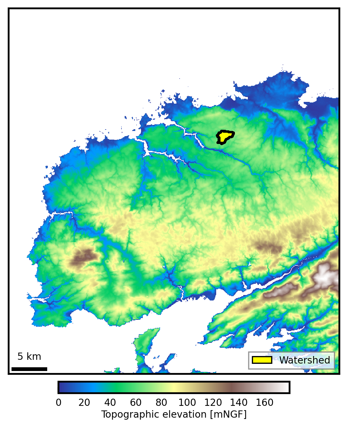
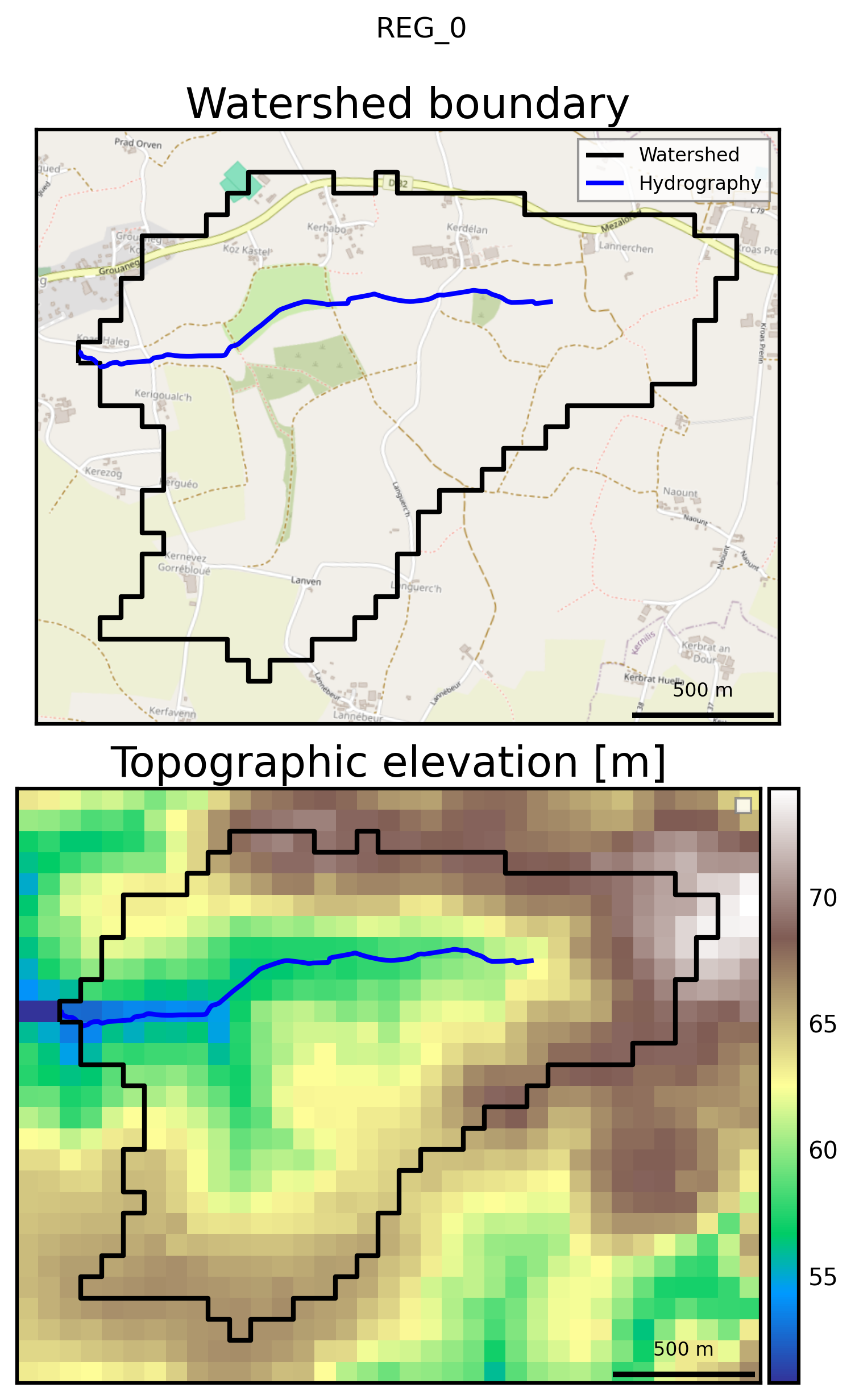
print('PLOT: WATERSHED INFO')

# General plot of the study site
visualization_watershed.watershed_local(dem_path, BV)
visu = visualization_results.Visualization(BV, model_name)
visu.visual2D(object_list = ['map','grid'], color_scale = [(None,None),(None,None)], lines=None)
PLOT: WATERSHED INFO
[INFO] Plotting 2D map visualizations for model reg_0
[14]:
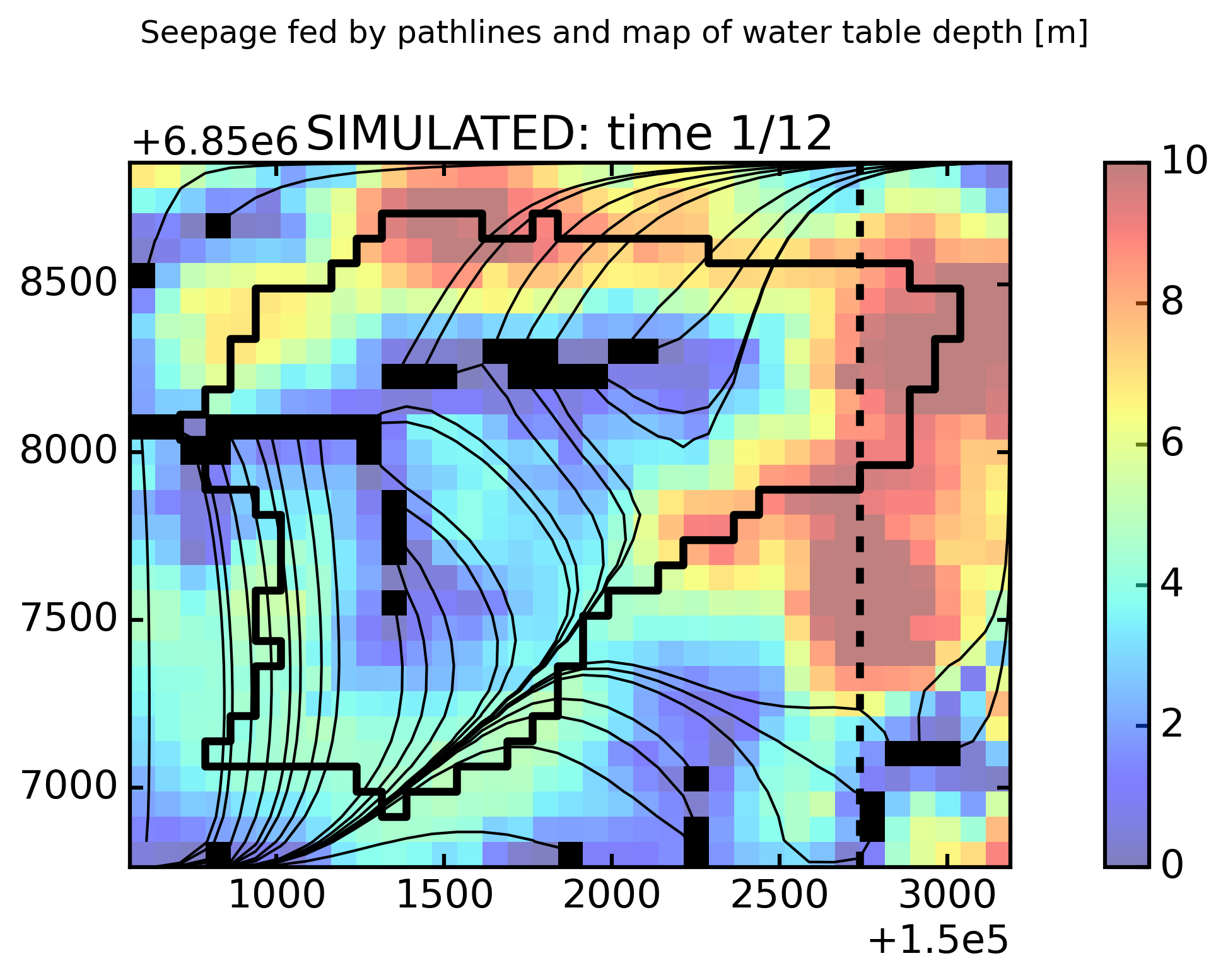
print('PLOT: MAPS')

fig, ax = plt.subplots(1,1, figsize=(8, 5), dpi=300)

sim_wtd = rasterio.plot.show(sim_wtd_data, ax=ax, transform=sim_wtd_rio.transform, cmap='jet',
                             vmin=0, vmax=10, alpha=0.5, zorder=0, aspect="auto")
rasterio.plot.show(sim_seep_data, ax=ax, transform=sim_seep_rio.transform, cmap=mpl.colors.ListedColormap(['k']), alpha=1, zorder=1, aspect="auto")
sim_contour.plot(ax=ax, lw=3, ec='k', fc='None')
sim_pathlines.plot(ax=ax, color='k')
ax.set_title('SIMULATED: time 1/12')
im = sim_wtd.get_images()[0]
divider = make_axes_locatable(ax)
cax = divider.append_axes('right', size='5%', pad=0.5)
fig.colorbar(im, cax=cax)
ax.axvline(x=ax.get_xlim()[0]+((29)*75), color='k', ls='--', lw=3)

fig.suptitle('Seepage fed by pathlines and map of water table depth [m]', y=1.02, fontsize=12)
fig.tight_layout()
PLOT: MAPS
[15]:
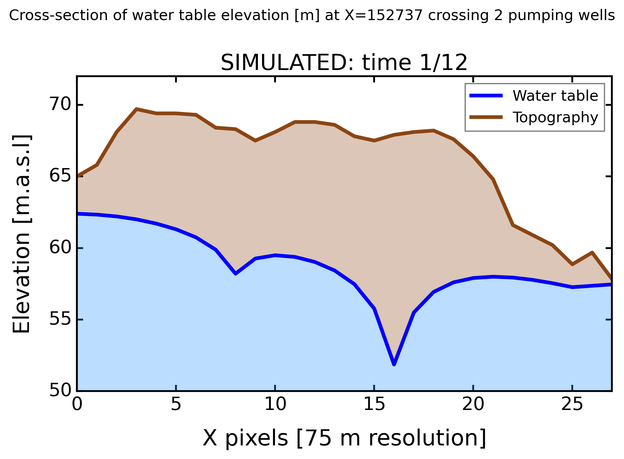
print('PLOT: CROSS-SECTION')

fig, ax = plt.subplots(1,1, figsize=(7, 5), dpi=300)

x_sim_wte = np.arange(0,sim_wte_data.shape[0],1)
y_sim_wte = sim_wte_data[:,28:29]
y_sim_wte = np.concatenate(y_sim_wte, axis=0)
ax.fill_between(x_sim_wte, x_sim_wte*0, y_sim_wte, lw=0, alpha=0.3, color='dodgerblue')
ax.plot(x_sim_wte, y_sim_wte, lw=3, color='blue', label='Water table')

x_sim_dem = np.arange(0,sim_dem_data.shape[0],1)
y_sim_dem = sim_dem_data[:,28:29]
y_sim_dem = np.concatenate(y_sim_dem, axis=0)
ax.fill_between(x_sim_dem, y_sim_wte, y_sim_dem, lw=0, alpha=0.3, color='saddlebrown')
ax.plot(x_sim_dem, y_sim_dem, lw=3, color='saddlebrown', label='Topography')

ax.set_xlim(0,27)
ax.set_ylim(50,72)
ax.legend(prop={'size': 12})
ax.set_xlabel('X pixels [75 m resolution]')
ax.set_ylabel('Elevation [m.a.s.l]')
ax.set_title('SIMULATED: time 1/12')

fig.suptitle('Cross-section of water table elevation [m] at X=152737 crossing 2 pumping wells', y=1.02, fontsize=12)
fig.tight_layout()
PLOT: CROSS-SECTION
[16]:
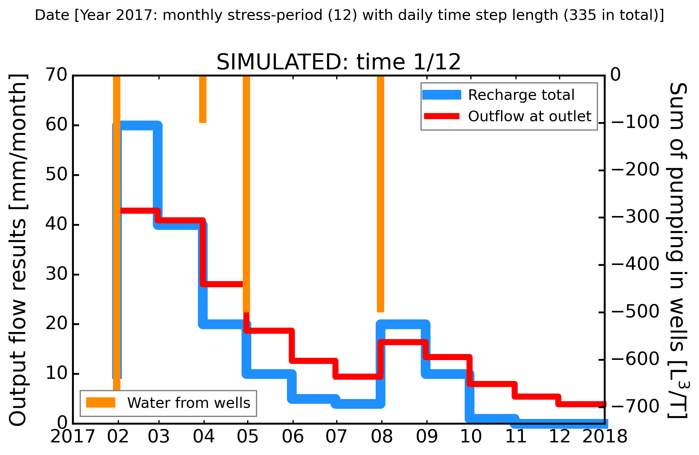
print('PLOT: GRAPHS')

well_1_fluxes_plot = well_1_fluxes.copy()
well_1_fluxes_plot.index = sim_timeseries.index
well_2_fluxes_plot = well_2_fluxes.copy()
well_2_fluxes_plot.index = sim_timeseries.index
well_all_fluxes_plot = well_1_fluxes_plot + well_2_fluxes_plot

fig, ax = plt.subplots(1, 1, figsize=(8, 5), dpi=300)

axb = ax.twinx()
ax.step(sim_timeseries.index, sim_timeseries['recharge']*30*1000, lw=8, color='dodgerblue', label='Recharge total', where='pre', clip_on=False)
ax.step(sim_timeseries.index, sim_timeseries['outflow_drain']*30*1000, lw=5, color='red', alpha=1, label='Outflow at outlet', where='pre', clip_on=False)
ax.set_xlim(pd.to_datetime('2017-01'), pd.to_datetime('2018-01'))
ax.set_ylabel('Output flow results [mm/month]')
ax.set_ylim(0, 70)
ax.xaxis.set_major_locator(mdates.YearLocator())
ax.xaxis.set_minor_locator(mdates.MonthLocator())
ax.xaxis.set_minor_formatter(mdates.DateFormatter('%m'))
ax.legend(prop={'size': 12})
axb.bar(sim_timeseries.index, well_all_fluxes_plot, clip_on=False, width=5, lw=0, color='darkorange', label='Water from wells')
# axb.set_ylim(-110,0)
axb.set_ylabel('Sum of pumping in wells [L$^3$/T]', rotation=270, labelpad=25)
ax.set_title('SIMULATED: time 1/12')
axb.legend(prop={'size': 12}, loc='lower left', facecolor='white')

fig.suptitle('Date [Year 2017: monthly stress-period (12) with daily time step length (335 in total)]', y=1.02, fontsize=12)
fig.tight_layout()
PLOT: GRAPHS
[17]:
os.chdir(root_dir)

# %%