
Exponential Distribution Of Residence Times#
[2]:
# -*- coding: utf-8 -*-
"""
 * Copyright (c) 2023 Alexandre Gauvain, Ronan Abhervé, Jean-Raynald de Dreuzy
 *
 * This program and the accompanying materials are made available under the
 * terms of the Eclipse Public License 2.0 which is available at
 * http://www.eclipse.org/legal/epl-2.0, or the Apache License, Version 2.0
 * which is available at https://www.apache.org/licenses/LICENSE-2.0.
 *
 * SPDX-License-Identifier: EPL-2.0 OR Apache-2.0
"""
[2]:
'\n * Copyright (c) 2023 Alexandre Gauvain, Ronan Abhervé, Jean-Raynald de Dreuzy\n *\n * This program and the accompanying materials are made available under the\n * terms of the Eclipse Public License 2.0 which is available at\n * http://www.eclipse.org/legal/epl-2.0, or the Apache License, Version 2.0\n * which is available at https://www.apache.org/licenses/LICENSE-2.0.\n *\n * SPDX-License-Identifier: EPL-2.0 OR Apache-2.0\n'
[3]:
# Libraries installed by default
import sys
import os

import numpy as np
import pandas as pd

import geopandas as gpd
import matplotlib as mpl
import matplotlib.pyplot as plt
import flopy
import flopy.utils.binaryfile as fpu
import imageio
import rasterio as rio
from rasterio.transform import from_origin
from rasterio.warp import reproject
from rasterio.enums import Resampling
from scipy.optimize import curve_fit

import whitebox
wbt = whitebox.WhiteboxTools()
wbt.verbose = True

# ROOT DIRECTORY
from os.path import dirname, abspath
try:
    root_dir = '/home/bb/Documents/01_Git_Repository/01-HydroModPy-dev'
except NameError:
    root_dir = os.getcwd()
sys.path.append(root_dir)

# HYDROMODPY MODULES
from hydromodpy import watershed_root
from hydromodpy.display import visualization_watershed, visualization_results
from hydromodpy.tools import toolbox
fontprop = toolbox.plot_params(8,15,18,20)  # small, medium, interm, large

def select_period(df, first, last):
    df = df[(df.index.year>=first) & (df.index.year<=last)]
    return df
[4]:
example_path = os.path.join(root_dir, "examples", "08_exponential_distribution_of_residence_times/")
data_path = os.path.join(example_path, "data/")

# The folder out_path is created in the example_path root directory:
out_path = os.path.join(root_dir,'examples', 'results')
# Or define it manually
# out_path = 'C:/Simulations/HydroModPy/'

print('The results of the example will be saved here :', out_path)
The results of the example will be saved here : /home/bb/Documents/01_Git_Repository/01-HydroModPy-dev/examples/results
[5]:
dL_fact = 0.01              # ratio between thickness and lenght of the aquifer d/L
dx = 10                     # discretization in the x-axis
part_num = 1                # particle number per cell
tracking_dir = 'forward'    # 'backward'

model_name = 'test_v1'
[6]:
case = 'Example_08_Synthetic'         #name of the folder in examples folder

if case == 'Example_08_Synthetic':
    dem_path_ref = data_path + 'hillslope_1D.tif'

    resamp_res = dx
    dem_path_res = data_path + 'hillslope_1D_resampled'+str(resamp_res)+'.tif'

    if not os.path.exists(dem_path_res):
        # open reference file and get resolution
        x_res = resamp_res
        y_res = resamp_res  # make sure this value is positive
        # specify input and output filenames
        inputFile = dem_path_ref
        outputFile = dem_path_res
        # resample the raster to the desired resolution
        with rio.open(inputFile) as src:
            dst_transform = from_origin(
                src.bounds.left,
                src.bounds.top,
                x_res,
                y_res
            )
            dst_width = max(1, int(np.ceil((src.bounds.right - src.bounds.left) / x_res)))
            dst_height = max(1, int(np.ceil((src.bounds.top - src.bounds.bottom) / y_res)))
            dst_meta = src.meta.copy()
            dst_meta.update({
                "driver": "GTiff",
                "transform": dst_transform,
                "width": dst_width,
                "height": dst_height
            })
            with rio.open(outputFile, "w", **dst_meta) as dst:
                for band in range(1, src.count + 1):
                    reproject(
                        source=rio.band(src, band),
                        destination=rio.band(dst, band),
                        src_transform=src.transform,
                        src_crs=src.crs,
                        dst_transform=dst_transform,
                        dst_crs=src.crs,
                        resampling=Resampling.bilinear
                    )

    x = imageio.imread(dem_path_res)
    x = (x*0)+1000*dL_fact
    toolbox.export_tif(dem_path_res, x, data_path + 'hillslope_1D_userdefined.tif', -99999)
    dem_path = data_path + 'hillslope_1D_userdefined.tif'

    load = False
    watershed_name = case
    from_lib = None # os.path.join(root_dir,'watershed_library.csv')
    from_dem = [dem_path, 10] # [path, cell size]
    from_shp = None # [path, buffer size]
    from_xyv = None # [x, y, snap distance, buffer size]
    bottom_path = None # path
    modflow_path = os.path.join(root_dir,'bin/')
    save_object = True
[7]:
print('##### '+watershed_name.upper()+' #####')

# load = True
BV = watershed_root.Watershed(dem_path=dem_path,
                              out_path=out_path,
                              load=load,
                              watershed_name=watershed_name,
                              from_lib=from_lib, # os.path.join(root_dir,'watershed_library.csv')
                              from_dem=from_dem, # [path, cell size]
                              from_shp=from_shp, # [path, buffer size]
                              from_xyv=from_xyv, # [x, y, snap distance, buffer size]
                              bottom_path=bottom_path, # path
                              save_object=save_object)

# Paths generated automatically but necessary for plots
stable_folder = out_path+'/'+watershed_name+'/'+'results_stable/'
simulations_folder = out_path+'/'+watershed_name+'/'+'results_simulations/'
[INFO]       __  __          __           __  ____          ________
[INFO]      / / / /         / /          /  \/   /         / / __  /
[INFO]     / /_/ /_  ______/ /________  /       /___  ____/ / /_/ /_  __
[INFO]    / __  / / / / __  / ___/ __ \/ /\,-/ / __ \/ __  / ____/ / / /
[INFO]   / / / / /_/ / /_/ / /  / /_/ / /   / / /_/ / /_/ / /   / /_/ /
[INFO]  /_/ /_/\__, /_____/_/   \____/_/   /_/\____/_____/_/____\__, /
[INFO]        /____/ Hydrological Modelling in Python /_____________/
[INFO]
[INFO] Initializing watershed object from scratch as requested
[INFO] Extracting geographic data for model area
##### EXAMPLE_08_SYNTHETIC #####
[8]:
# Frame settings
box = True # or False
sink_fill = False # or True
sim_state = 'steady' # 'steady' or 'transient'
plot_cross = False
dis_perlen =  True
check_grid = True

# Ratio to reach
KR = 15000 # hydraulic conductivity divided by recharge
# KR = 10 # hydraulic conductivity divided by recharge

# Climatic settings
recharge = 1 / 1000 # 33 mm/day
first_clim = 'mean'

# Hydraulic settings
hk = KR * recharge
nlay = 10
lay_decay = 1 # 1 for no decay
bottom = 0 # elevation in meters, None for constant auifer thickness, or 2D matrix
thick = 1000*dL_fact # if bottom is None, aquifer thickness
hk_decay = 0 # exponential decay : 1/20 (half decrease at 20m)
cond_drain = 0 # if 0, DRN is not actvated, with None: linked to hk value of the first layer
sy = 10 / 100 # -
ss = 1e-10

# Boundary settings
bc_left = 5 # or value
# bc_left = thick # or value
bc_right = None # or value
sea_level = 'None' # or value based on specific data : BV.oceanic.MSL
[9]:
# Import modules
BV.add_settings()
BV.add_climatic()
BV.add_hydraulic()

# Frame settings
BV.settings.update_model_name(model_name)
BV.settings.update_box_model(box)
BV.settings.update_sink_fill(sink_fill)
BV.settings.update_simulation_state(sim_state)
BV.settings.update_check_model(plot_cross=plot_cross, check_grid=check_grid)

# Climatic settings
BV.climatic.update_recharge(recharge, sim_state=sim_state)
BV.climatic.update_first_clim(first_clim)

# Hydraulic settings
BV.hydraulic.update_nlay(nlay) # 1
BV.hydraulic.update_lay_decay(lay_decay) # 1
BV.hydraulic.update_bottom(bottom) # None
BV.hydraulic.update_thick(thick) # 30 / intervient pas si bottom != None
BV.hydraulic.update_hk(hk)
BV.hydraulic.update_sy(sy)
BV.hydraulic.update_ss(ss)

# Boundary settings
BV.settings.update_bc_sides(bc_left, bc_right)
BV.add_oceanic(sea_level)
BV.settings.update_dis_perlen(dis_perlen)
[INFO] Initializing settings module for groundwater parameters
[INFO] Initializing climatic module parameters
[INFO] Initializing hydraulic module for parameter setup
[10]:
model_modflow = BV.preprocessing_modflow(for_calib=False)
success_modflow = BV.processing_modflow(model_modflow, write_model=True, run_model=True)

BV.postprocessing_modflow(model_modflow,
                          watertable_elevation = True,
                          watertable_depth= True,
                          seepage_areas = True,
                          outflow_drain = True,
                          groundwater_flux = True,
                          groundwater_storage = True,
                          accumulation_flux = True,
                          persistency_index = False,
                          intermittency_monthly = False,
                          intermittency_daily = False,
                          export_all_tif = False)

BV.settings.update_input_particles(zone_partic = BV.geographic.watershed_dem,
                                    cell_div = part_num, # 1, distribution of partciles by cell in x and y direction
                                    zloc_div = False,  # False or True, inject partciles in z direction. Same number as cell_div
                                    bore_depth = None, # None or True, None 1 particle in the first layer, If True it will inject 1 particle in every layer.
                                    track_dir = tracking_dir, # backward or forward
                                    sel_random = None, # or int
                                    sel_slice = None, # or int
                                    )

model_modpath = BV.preprocessing_modpath(model_modflow)
success_modpath = BV.processing_modpath(model_modpath, write_model=True, run_model=True)

BV.postprocessing_modpath(model_modpath,
                          ending_point=True,
                          starting_point=True,
                          pathlines_shp=True,
                          particles_shp=True,
                          random_id=None) # None

BV.filtprocessing_modpath(model_modpath,
                          norm_flux=True, # for forward only
                          filt_time=True, # delete particles with time at 0, add a column with time divided by 365 (considering recharge in days)
                          filt_seep=False, # only forward, keep only particles finishing in zone1 (seepage), keep only particles finishing in k1 (first layer)
                          filt_inout=True, # delete particles in and out in the same cell (first layer)
                          calc_rtd=True, # compute residence time distribution
                          random_id=None, # select randomly to keep
                          ) # None
[INFO] MODFLOW grid connectivity check passed
FloPy is using the following executable to run the model: ../../../../../bin/linux/mfnwt

                                  MODFLOW-NWT-SWR1
    U.S. GEOLOGICAL SURVEY MODULAR FINITE-DIFFERENCE GROUNDWATER-FLOW MODEL
                             WITH NEWTON FORMULATION
                             Version 1.3.0 07/01/2022
                    BASED ON MODFLOW-2005 Version 1.12.0 02/03/2017

                    SWR1 Version 1.05.0 03/10/2022

 Using NAME file: test_v1.nam
 Run start date and time (yyyy/mm/dd hh:mm:ss): 2025/11/12  1:42:51

 Solving:  Stress period:     1    Time step:     1    Groundwater-Flow Eqn.
[INFO] Post-processing stress period 1/1
 Run end date and time (yyyy/mm/dd hh:mm:ss): 2025/11/12  1:42:52
 Elapsed run time:  0.422 Seconds

  Normal termination of simulation
[INFO] Exporting watertable elevation time series
[INFO] Exporting watertable depth time series
[INFO] Exporting seepage areas time series
[INFO] Exporting outflow drain time series
[INFO] Exporting groundwater flux time series
[INFO] Exporting groundwater storage time series
[INFO] Exporting accumulation flux time series
writing loc particle data
FloPy is using the following executable to run the model: ../../../../../bin/linux/mp6
Processing basic data ...
Checking head file ...
Checking budget file and building index ...

Run particle tracking simulation ...
Processing Time Step     1 Period     1.  Time =  1.00000E+00
Particle tracking complete. Writing endpoint file ...
End of MODPATH simulation. Normal termination.
(numpy.record, [('particleid', '<i4'), ('particlegroup', '<i4'), ('timepointindex', '<i4'), ('cumulativetimestep', '<i4'), ('time', '<f4'), ('x', '<f4'), ('y', '<f4'), ('z', '<f4'), ('k', '<i4'), ('i', '<i4'), ('j', '<i4'), ('grid', '<i4'), ('xloc', '<f4'), ('yloc', '<f4'), ('zloc', '<f4'), ('linesegmentindex', '<i4')])
(numpy.record, [('particleid', '<i4'), ('particlegroup', '<i4'), ('timepointindex', '<i4'), ('cumulativetimestep', '<i4'), ('time', '<f4'), ('x', '<f4'), ('y', '<f4'), ('z', '<f4'), ('k', '<i4'), ('i', '<i4'), ('j', '<i4'), ('grid', '<i4'), ('xloc', '<f4'), ('yloc', '<f4'), ('zloc', '<f4'), ('linesegmentindex', '<i4')])
[11]:
# Load model
fname = simulations_folder+model_name+'/'+model_name
ml = flopy.modflow.Modflow.load(fname+'.nam')
hdobj = flopy.utils.HeadFile(fname + '.hds')
times = hdobj.get_times()
for i, t in enumerate([times[0]]):
# Data
i = int(i)
head = hdobj.get_data(totim=t)
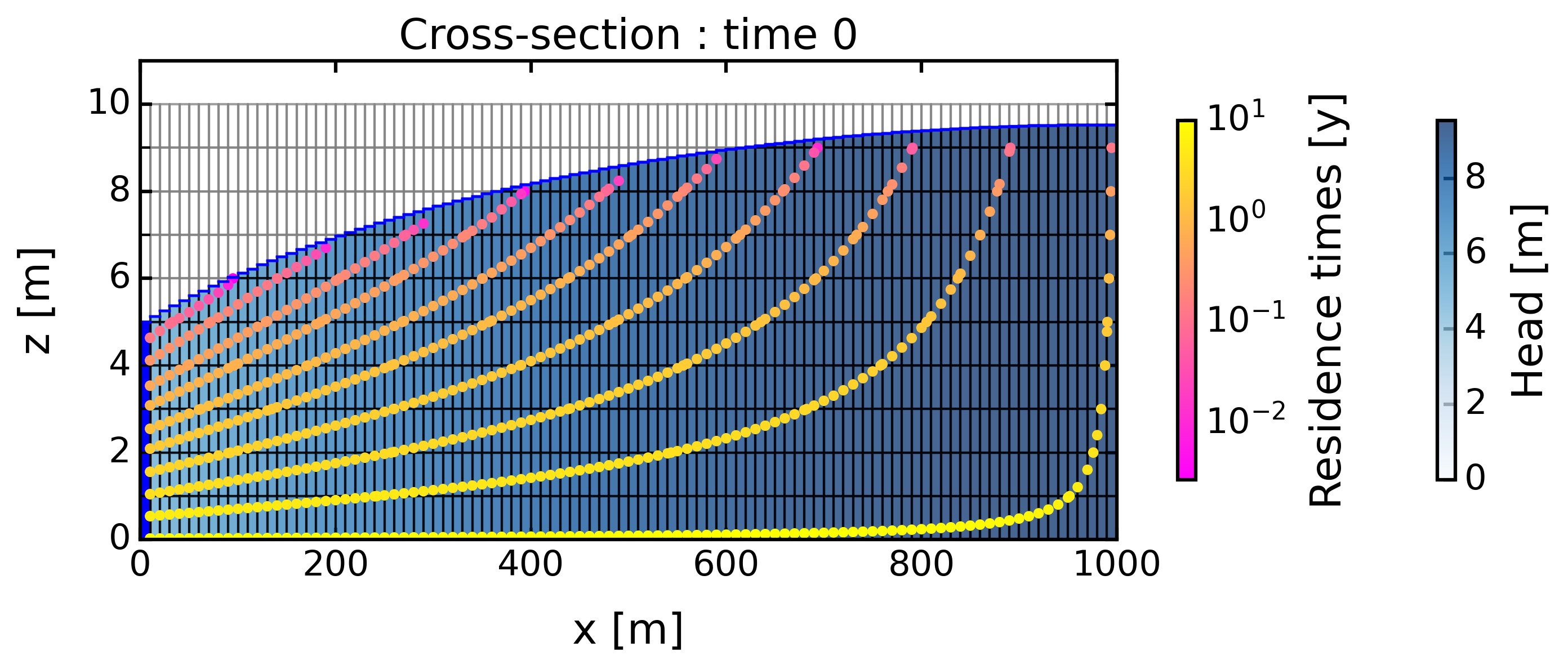
# Figure
fig = plt.figure(figsize=(10, 4), dpi=300)
ax = fig.add_subplot(1, 1, 1)
ax.set_title('Cross-section : '+'time '+str(i))
ax.set_xlabel('x [m]')
ax.set_ylabel('z [m]')
# Init cross-section
xsect = flopy.plot.PlotCrossSection(model=ml, line={'Row': 0})
# Head color
pc = xsect.plot_array(head, masked_values=[999.], head=head, cmap='Blues',
vmin=0, vmax=None,
alpha=0.75)
cb = plt.colorbar(pc, shrink=0.75)
cb.set_label('Head [m]', labelpad=+10)
wt = xsect.plot_surface(head, masked_values=[999.], color='b', lw=1)
# Boundary
patches = xsect.plot_ibound(head=head)
# Grid
linecollection = xsect.plot_grid(alpha=0.75, zorder=0)
# # Particles plot
end = gpd.read_file(simulations_folder+model_name+'/_postprocess/_particles/ending.shp')
prt = gpd.read_file(simulations_folder+model_name+'/_postprocess/_particles/particles.shp')
# list_particles = end[end['i0']==1]['particleid'].unique()
### Filtering if necessary
# shp_fil = shp.copy()
# shp_fil = shp[shp['zone']==1]
# shp_fil = shp[shp['time']>1]
# shp_fil = shp_fil[shp_fil['particleid'].isin(list_particles)]
list_particles = [10,20,30,40,50,60,70,80,90,100]
# prt_fil = prt[prt['particleid']==100]
prt_fil = prt[prt['particleid'].isin(list_particles)]
sc = ax.scatter(prt_fil['x'], prt_fil['z'], c=prt_fil['time']/365, s=20,
cmap='spring', linewidths=0, norm=mpl.colors.LogNorm(vmin=1/365, vmax=10))
cbsc = plt.colorbar(sc, shrink=0.75)
cbsc.set_label('Residence times [y]', labelpad=+10)
# Adjust
ax.set_ylim(0,thick*1.1)
fig.tight_layout()
[12]:
# Data
end = gpd.read_file(BV.geographic.simulations_folder+'/'+model_name+'/'+'_postprocess/_particles/'+'ending_weighted.shp')
end[end['time_win_y']==0] = np.nan
end = end.dropna()
# Tau
if tracking_dir == 'forward':
tau = np.average(end['time_win_y'], weights=end['rchPerc'])
else:
tau = np.average(end['time_win_y'])
# Pdf
def pdf_function(M, nbin, Weight):
bin_min = np.quantile(M, 0.01)
bin_max = np.quantile(M, 0.99)
bins = np.logspace(np.log10(bin_min),np.log10(bin_max), nbin)
pdf, binEdges = np.histogram(M, bins=bins, density=True, weights=Weight)
dx = np.diff(binEdges)
xh = (binEdges[1:] + binEdges[:-1])/2
xh = np.array(xh)
return (xh, pdf)
# Bin
nbin = int(2*len(end['time_win_y'])**(2/5)) #Scott's Rules
if tracking_dir == 'forward':
[xh, yh] = pdf_function(end['time_win_y']/tau, nbin, end['rchPerc'])
else:
[xh, yh] = pdf_function(end['time_win_y']/tau, nbin, np.ones(len(end)))
# Log
idzeros = np.where(yh != 0)
xfil = xh[idzeros]
yfil = yh[idzeros]
x_log = np.log10(xfil)
y_log = np.log10(yfil)
# Fit
def func(x, a, b, c, d, e):
return a * x**4 + b * x**3 + c * x**2 + d * x + e
params, covariance = curve_fit(func, x_log, y_log)
a, b, c, d, e = params
x_fit = np.linspace(min(x_log), max(x_log), 100)
y_fit = func(x_fit, a, b, c, d, e)
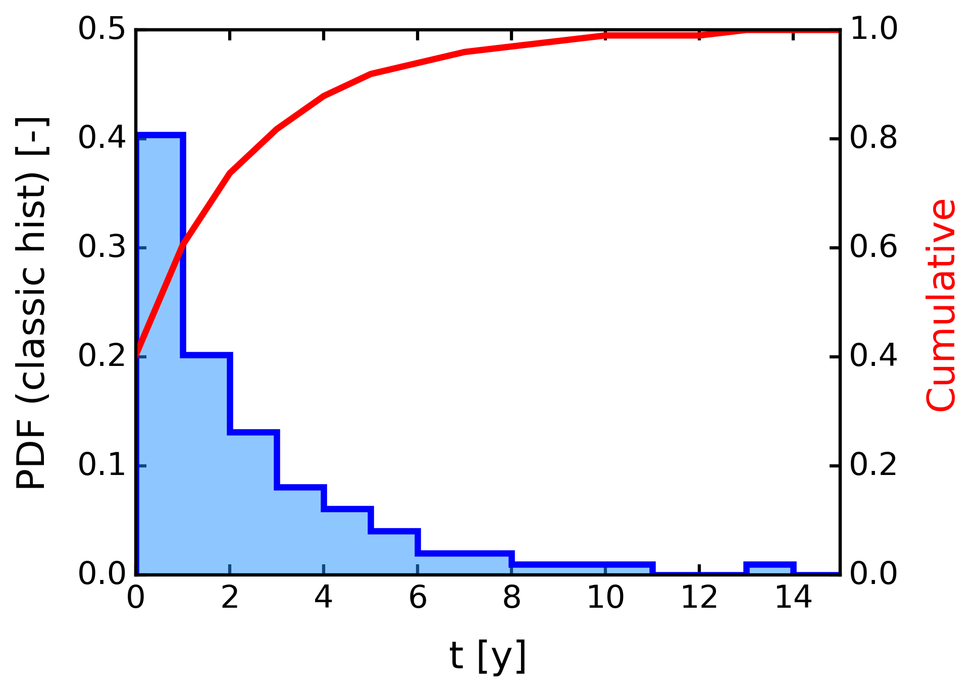
# PLot 1
fig = plt.figure(figsize=(6,4.5))
ax = fig.add_subplot(111)
axb = ax.twinx()
counts, bins = np.histogram(end['time_win_y'], density=True, weights=end['rchPerc'], bins=range(100))
ax.hist(end['time_win_y'], density=True, bins=range(100), weights=end['rchPerc'], facecolor='dodgerblue', alpha=0.5, lw=0)
ax.stairs(counts, bins, lw=3, color='b') # If the data has already been binned and counted, use bar or stairs to plot the distribution
ax.set_xlabel('t [y]')
ax.set_ylabel('PDF (classic hist) [-]')
ax.set_xlim(0, 15)
ax.set_ylim(0, 0.5)
axb.plot(bins[:-1], np.cumsum(counts), lw=3, ls='-', color='red')
axb.set_ylabel('Cumulative', color='red')
axb.set_ylim(0,1)
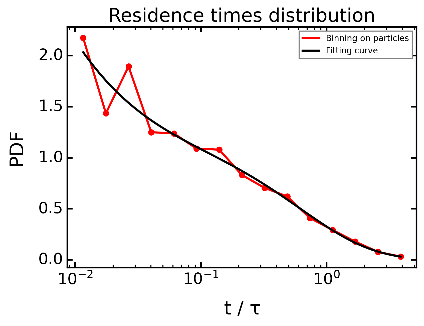
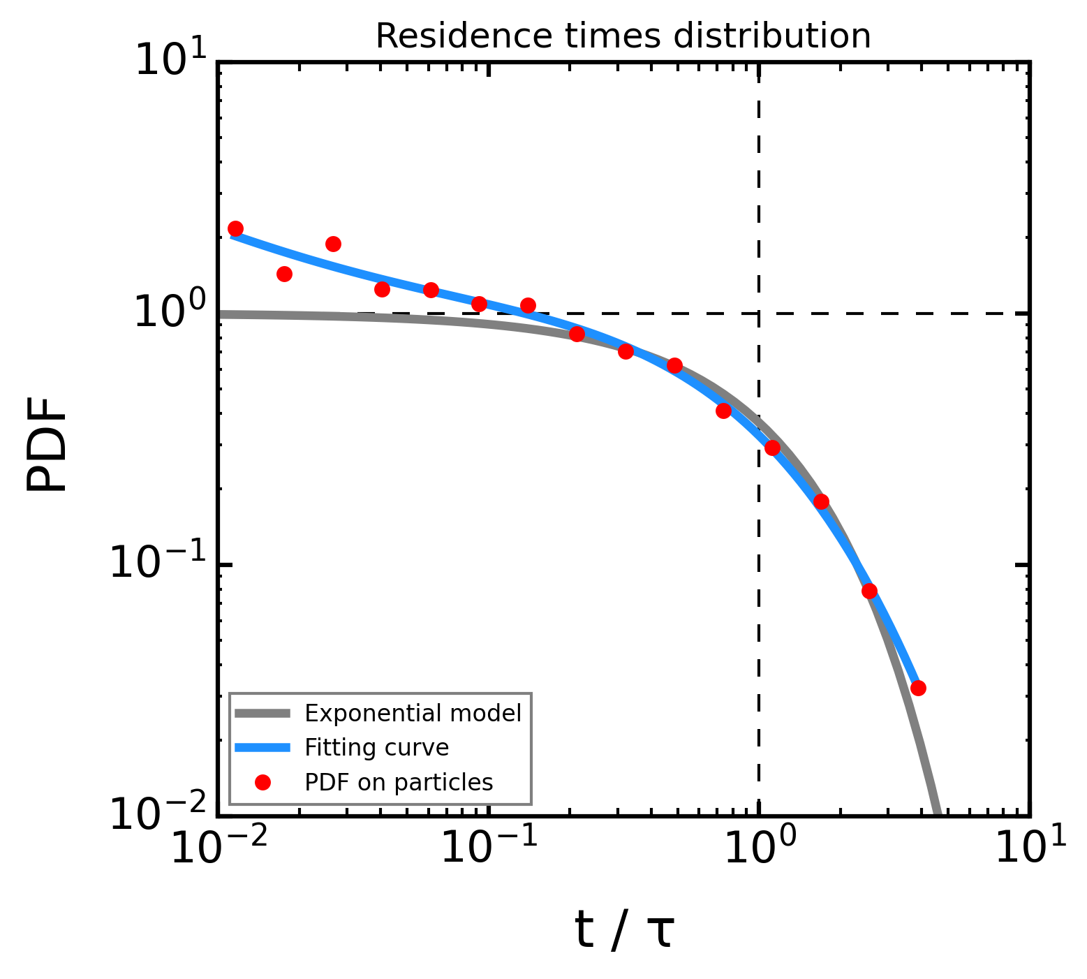
# Plot 2
fig = plt.figure(figsize=(5,4.5))
ax = fig.add_subplot(111)
tau2 = 1
t = np.logspace(-3, 1, 100)
p_ttd = 1/tau2*np.exp(-t/tau2)
ax.plot(t, p_ttd, 'grey', lw=3, label='Exponential model')
ax.plot(10**x_fit, 10**y_fit, '-', lw=3, c='dodgerblue', label='Fitting curve')
ax.plot(xh, yh, '.', lw=0, ms=10, c='red', label='PDF on particles')
intrp = np.interp(xh, t, p_ttd)
ax.set_ylabel("PDF")
ax.set_xlabel("t / "+r'$\tau$')
ax.set_xscale('log')
ax.set_yscale('log')
ax.set_title('Residence times distribution', fontsize=12)
ax.set_xlim(1e-2, 1e1)
ax.set_ylim(1e-2, 1e1)
ax.axvline(x=1, c='k', ls='--', zorder=-1)
ax.axhline(y=1, c='k', ls='--', zorder=-1)
ax.legend(loc='lower left')
[12]:
<matplotlib.legend.Legend at 0x775503009e50>
[13]:
# wbt.verbose = True
# wbt.resample(
#     dem_path_ref,
#     dem_path_res,
#     cell_size=100,
#     base=None,
#     method="cc")

# bx = fig.add_subplot(212)
# erro = (intrp - xh)/intrp * 100        # error calculus (teo - obs)/teo
# rms = np.sqrt(np.mean(erro**2))        # rms calculus
# bx.plot(xh, erro, 'o', label = 'RMS = '+ str(round(rms, 2)))
# bx.legend()
# bx.set_ylim(-100, 100)
# bx.set_xscale('log')
# bx.set_xlim(5e-3, 1.5e1)
# bx.set_xlim(0.5e-3, 1.5e1)